Deep Learning for Time Series
Deep learning is increasingly becoming a popular technique for analyzing time series data. Deep learning algorithms can be used to model and analyze time series data in various ways, including Recurrent Neural Networks (RNNs), Convolutional Neural Networks (CNNs), Long Short-Term Memory (LSTM), Autoencoders: Autoencoders, and Gated Recurrent Units (GRU). I will conduct RNN, LSTM, and GRU for this project, using homeownership rate data from 1980 to 2022.
Figure 1. Overview of Homeownership Rate Data, 1980-2022
Figure 2. Training and Testing Homeownership Rate Data Split, 1980-2022
RNN
RNNs are a type of neural network well-suited for modeling time series data. Unlike traditional feedforward neural networks, RNNs have loops in their architecture that allow them to maintain a "memory" of previous inputs. In an RNN, each time step receives an input and produces an output, fed into the next step. The input at each time step combines the current input and the output from the previous time step. This feedback loop allows the RNN to remember prior inputs and use this information to predict future inputs. One of the challenges with RNNs is the vanishing gradient problem, which occurs when gradients become very small during training, making it difficult to update the network's weights. Various modifications to the basic RNN architecture, such as Long Short-Term Memory (LSTM) and Gated Recurrent Unit (GRU) networks, have been developed. These modifications allow the RNN to handle long-term dependencies in the data better and mitigate the vanishing gradient problem.
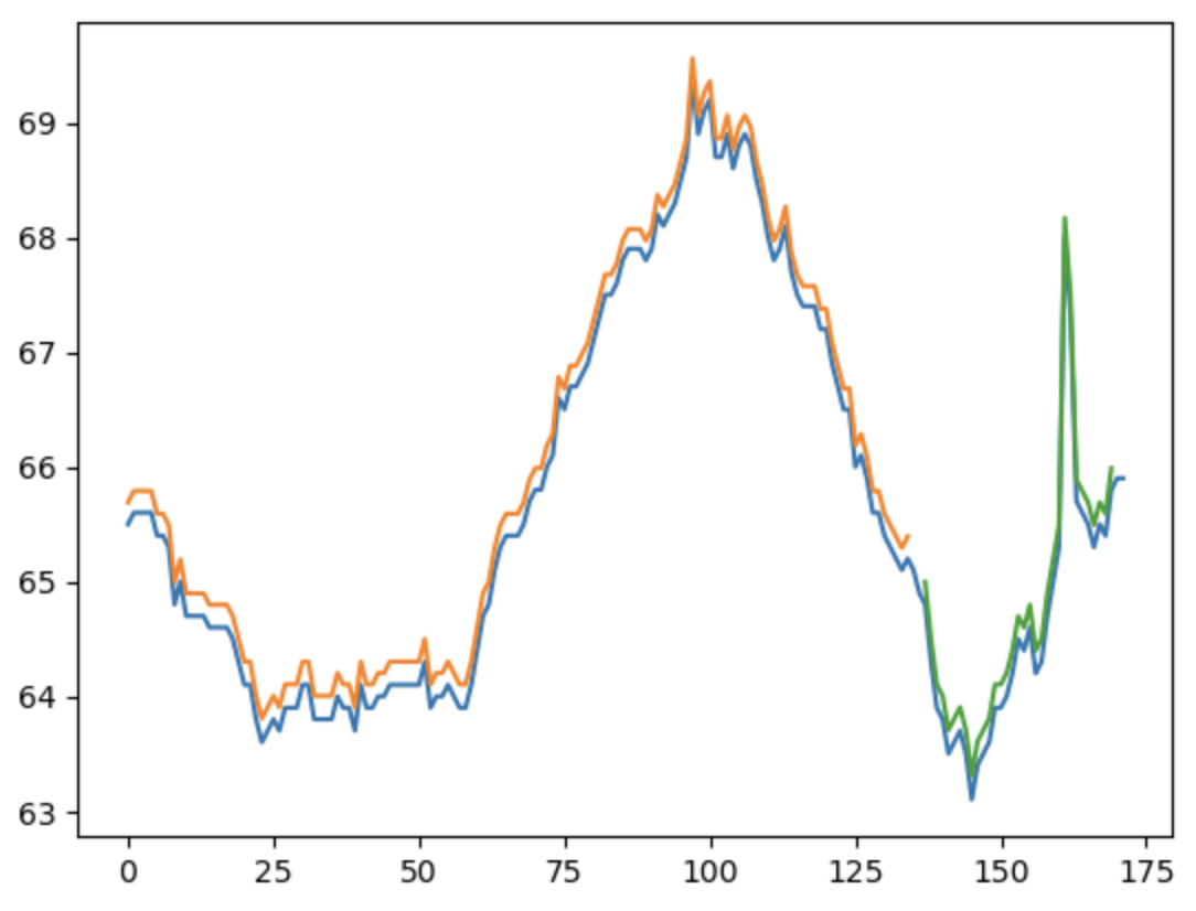
Train Score: 0.07 MSE (0.27 RMSE)
Test Score: 0.39 MSE (0.63 RMSE)
Figure 3:

LSTM
LSTM networks are particularly well-suited for modeling time series data because they can maintain a memory of previous inputs and selectively remember or forget information from prior time steps. For time series prediction, LSTMs are trained to predict the next value in a time series based on past values. The training is done by feeding the LSTM a sequence of past values and then predicting the next value. One of the critical advantages of LSTMs over traditional RNNs is their ability to handle long-term dependencies in the data, which can be particularly important for time series analysis tasks. LSTMs can learn to selectively remember or forget information from previous time steps, allowing them to maintain a memory of important information while discarding irrelevant information.
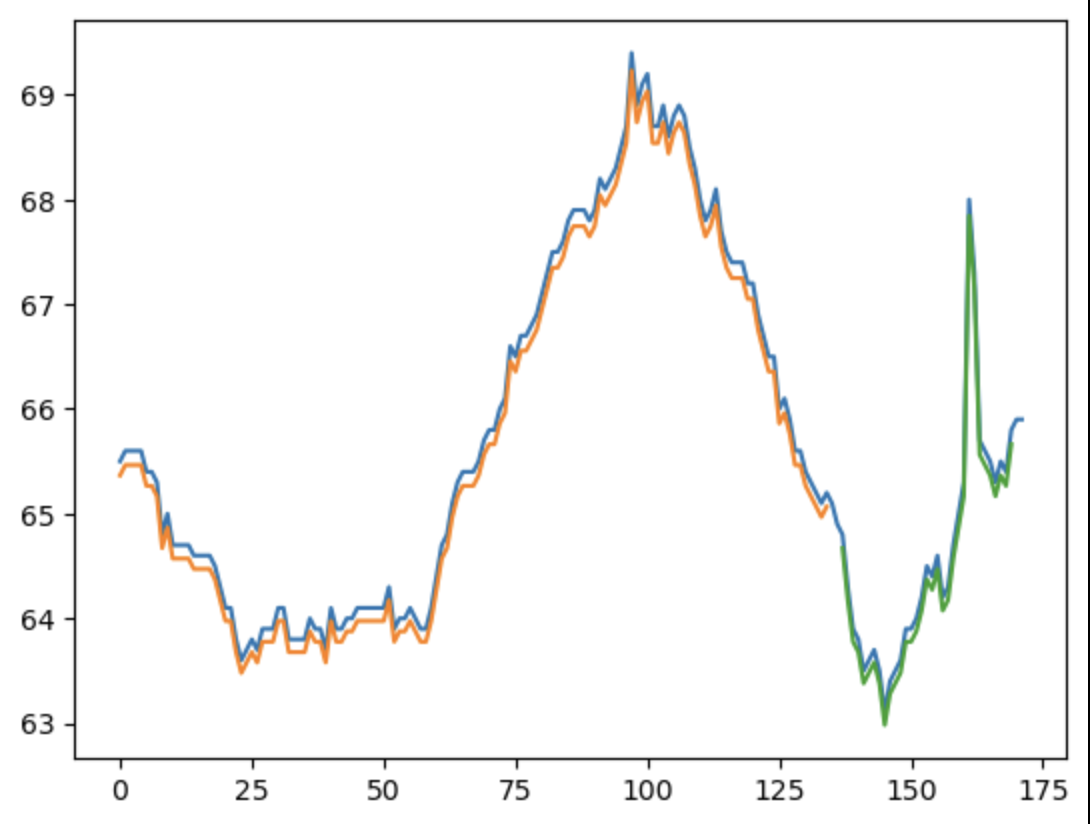
Train Score: 0.06 MSE (0.24 RMSE)
Test Score: 0.39 MSE (0.63 RMSE)
Figure 4.

GRU
GRU is a type of recurrent neural network (RNN) similar to LSTM. It is designed to address the same issues as LSTM, such as vanishing gradient, but with a simpler architecture. GRUs are widely used for time series analysis, particularly for sequence modeling, speech recognition, and machine translation tasks. The difference between GRU and LSTM is that GRU has only two gates: reset and update gates. These gates allow GRU to selectively forget or retain information from previous time steps, similar to LSTM. The reset gate determines how much of the prior hidden state should be used in the current time step, while the update gate determines how much of the new input and previous hidden state should be used to update the current hidden state. The architecture of a GRU is simpler than an LSTM, making it computationally less expensive to train. Some studies have shown that GRUs can perform as well as LSTMs on specific time series prediction tasks while requiring fewer parameters.
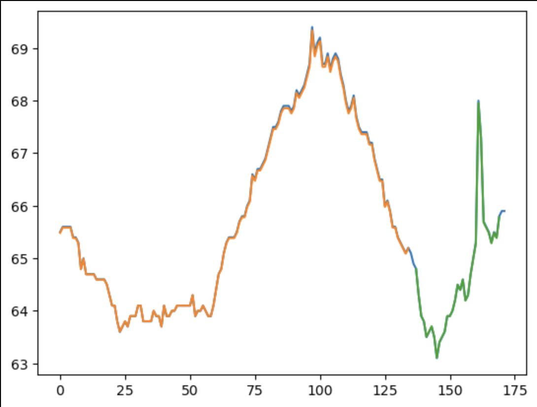
Train Score: 0.04 MSE (0.19 RMSE)
Test Score: 0.37 MSE (0.61 RMSE)
Figure 5.

Comparing the RMSE of RNN, LSTM, and GRU training errors, LSTM performs the best. However, looking at the testing errors of all three models, RNN has the lowest testing error; therefore, RNN performs the best compared to the three models. In all three models, the testing error was much larger than the training error, indicating and overfitting problem within the models.
Add regularizers to RNN
Using the "Add regularizers to RNN" method to avoid overfitting in RNN models. Regularization, which prevents the model from fitting the noise in the data and enhances generalization, involves adding a penalty term to the objective function during training. Regularization in RNNs can be applied to the network's weights or activations. L1 and L2 regularization, dropout, and early halting are a few regularization methods frequently employed in RNNs.
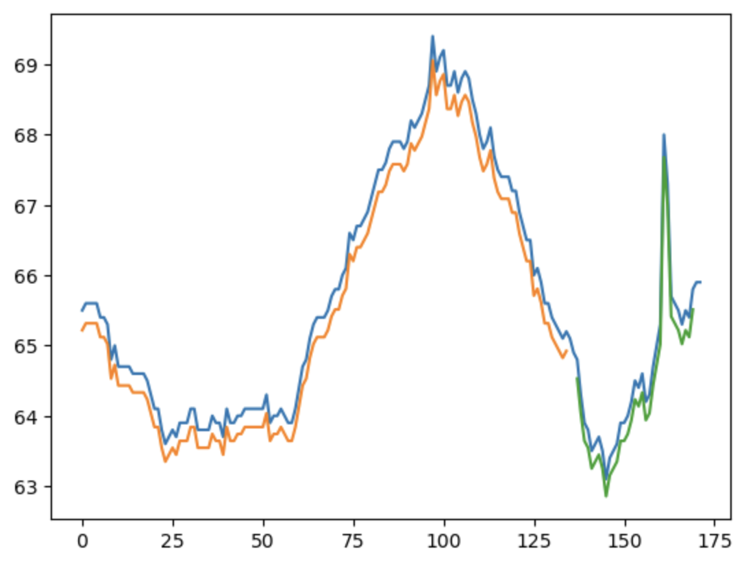
Train Score: 0.16 MSE (.40 RMSE)
Test Score: 0.50 MSE (.70 RMSE)
Figure 6.

As shown in figure 6, by using the "Add regularizer to RNN" method, we're able to improve the overfitting in RNN.
Summary
How do the results from the three different ANN models compare with each other in terms of accuracy and predictive power?
All three deep learning models were able to produce reasonably accurate predictions. The RNN model's performance is impressive because its ability to predict the index is near the actual value with a smaller RMSE than the other models. The remaining models are also good at predicting the change; thus, the anticipated test results are consistent with the initial data.
What effect does including regularization have on your results?
The L2 regulator with alpha=0.01 in the TensorFlow package was used to improve the overfitting problem. It could improve prediction accuracy by adding penalty terms to the loss function.
How far into the future can the deep learning model accurately predict the future?
The projected test data showed that the deep-learning models could accurately anticipate the outcome. However, the test data has a more significant error than the training data, indicating an overfitting problem. Because different models are fitted with varied complexity and data sizes, it is difficult to estimate how far they can be forecast.
How does your deep learning modeling compare to the traditional single-variable time-series ARMA/ARIMA models from HW-3?
The capacity of deep learning models to recognize non-linear correlations and dependencies in the data is one of its key advantages over conventional ARMA/ARIMA. To forecast highly non-linear and complicated time series, deep learning models can learn intricate patterns and relationships that regular models might not be able to capture. However, deep learning models frequently need much more data and computer power than conventional models, and the quantity and quality of the training data can significantly impact how well they function.