ARMA/ARIMA
ARMA (Autoregressive Moving Average) and ARIMA (Autoregressive Integrated Moving Average) are time series models used for forecasting future values of a variable based on its past values. The ARMA model combines the autoregressive (AR) and moving average (MA) components. The AR component represents the relationship between the current value of the variable and its past values. In contrast, the MA component represents the relationship between the present value of the variable and past errors (or residuals) of the model.The ARIMA model is an extension of the ARMA model that also includes a differencing component, which is used to remove trends or seasonal patterns from the time series data before applying the ARMA model. The differencing component is the "integrated" component of the model. ARMA and ARIMA models are widely used in econometrics, finance, and other fields for time series analysis and forecasting. These models can be used to model stationary and non-stationary time series data. They can be applied to various applications, such as stock market predictions and economic and weather forecasting. The models are typically estimated using maximum likelihood estimation or other statistical methods. Their accuracy can be evaluated using metrics such as mean squared error or root mean squared error.
In order to use a model such as ARMA, the time series must be stationary -one whose properties do not depend on the time at which the series is observed . the. If the time series is not stationary, we must differentiate or detrend the time series to make the series stationary. Therefore the first I model selection is first testing if the data is stationary. We do this by using the ACF plot – plots the correlation coefficient against the lag, which is measured in terms of a number of periods or units –and Augmented Dickey-Fuller (ADF) test. ADF test is used to check whether a given time series is at rest.
Figure 1a: APC Plot
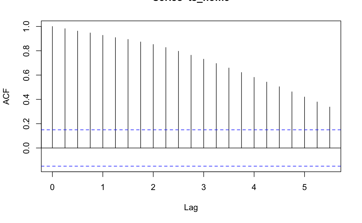
Figure 1b: ACF Test

Based on the figures about, both the ACF plot and the ADF test tell us that the time series is not stationary. The ACF plot shows that the correlation among the lag variables are significant so the data is not stationary. The ADF test also agrees with the ACF test, as the p-value is greater than 0.05. Based on these results we concluded that we need to difference the time series to make it stationary.
Diffrencing Data
Figure 2a: Diffrenced Time Series
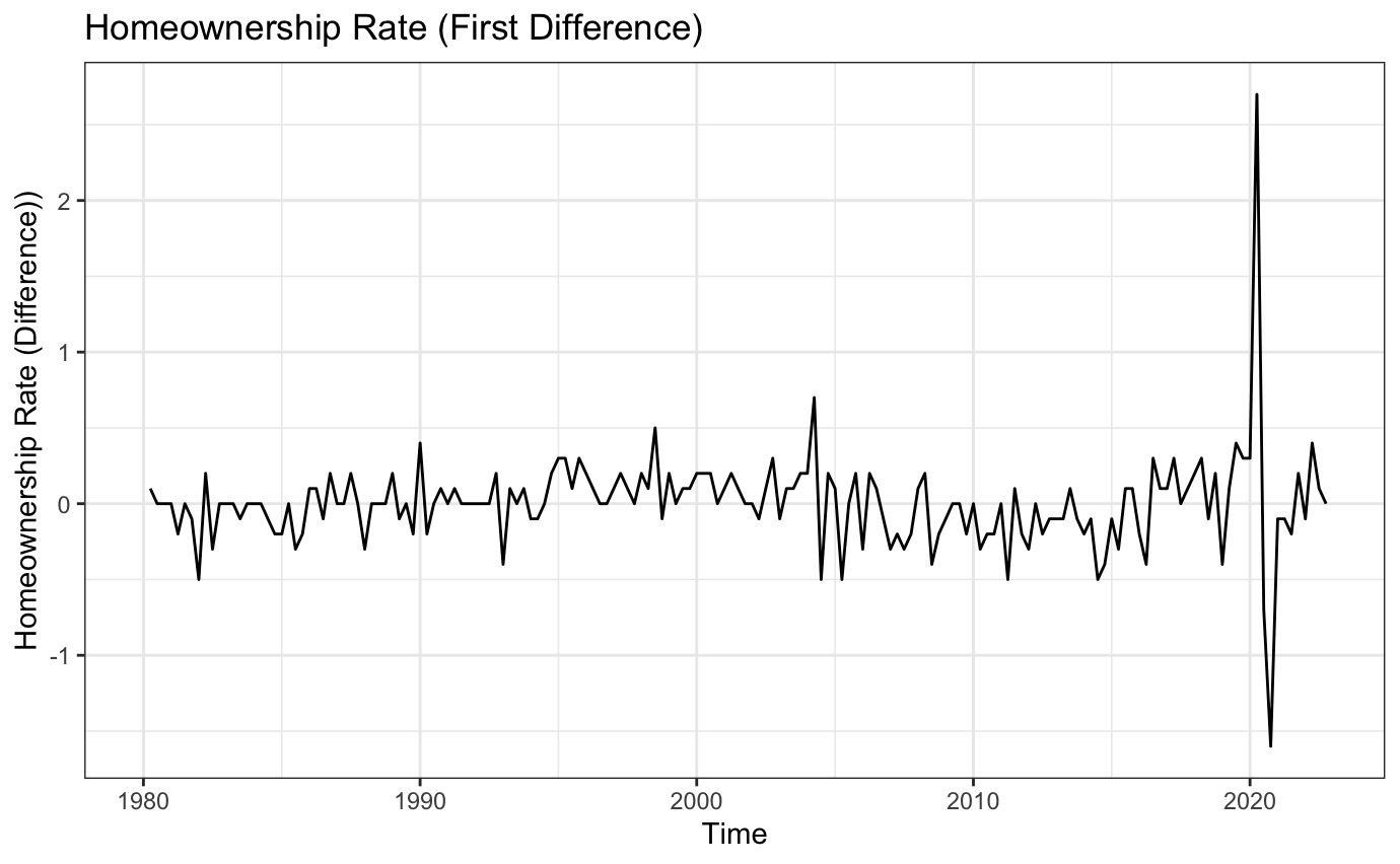
Figure 2b: ACF and PACF on Diffrenced Time Series
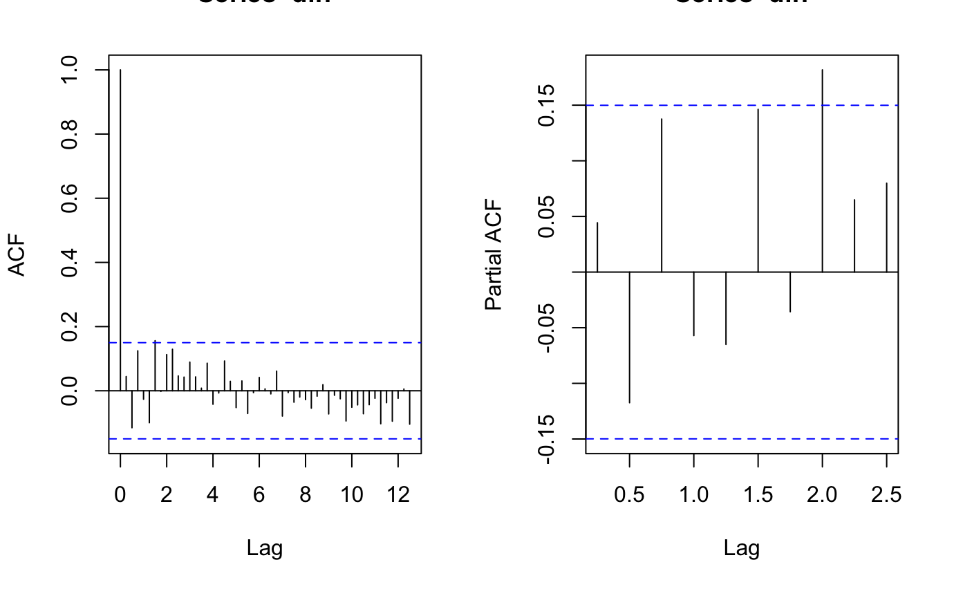
Figure 2c: ADF Test on Diffrenced Time Series

According to the plots above, the series is weakly stationary after the fist difference since the correlation among the lag variables are no longer significant. No more difference is needed.
Parameter Selection
Figure 3:ACF and PACF Plots for Homeownership Rates

Model Selection
We are now finding the best model with loops using the candidate parameters obtained from the last section. To compare each model, AIC, BIC, and AICc are used. AIC and BIC are used for model selection by trading off model complexity with the goodness of fit, with AIC placing a minor penalty on more complex models. AICc is a corrected version of AIC that is more appropriate for small sample sizes, as it sets a more significant penalty on more complex models.
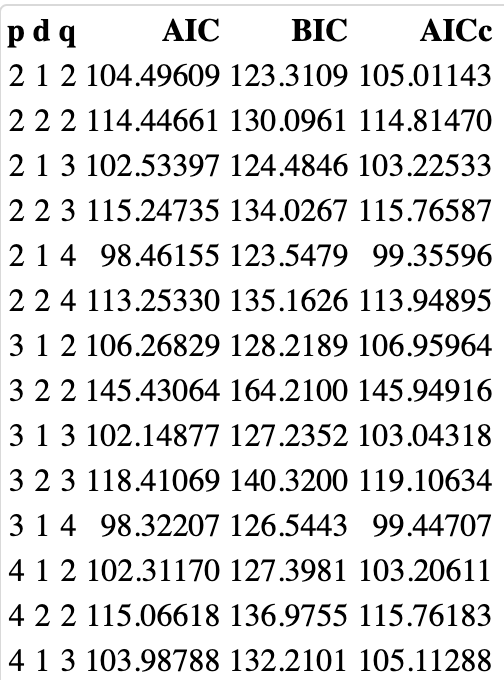
Below is a the output for the lowest AIC, BIC and AICc

The model with the lowerst AIC is model 11, with Arima(3,1,4). The model with the lowest BIC is model 1 with Arima(2,1,2). Lastly, the model with the lowest AICc is model 5 with Arima(2,1,4).Because model 1 has lowest number of AIC, BIC, and AICc of all three, ARIMA(2,1,2) is selected.
Model Diagnostics
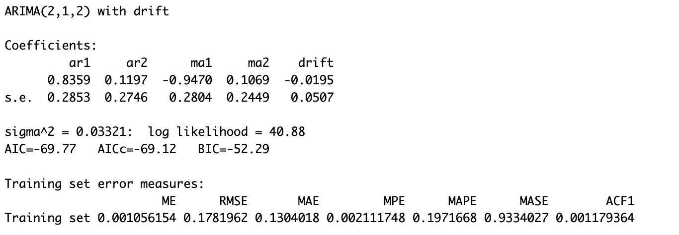
According to the ARIMA(2,1,2) model and the coefficients obtained by fitting. The function of the selected ARIMA model can be writen as: (1-B)(1-.83569 - .1197B2)Xt= -.0-195 + (1-.947B +.1069B2)Wt
Figure: Model 1 Model Diagnostics
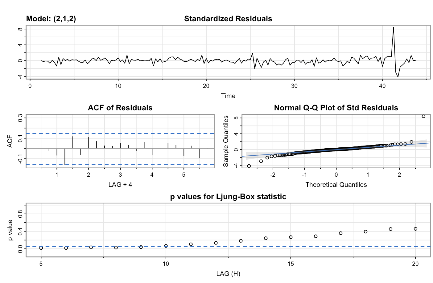
According to the residuals of the fitted model, the lags are not correlated, and the distribution of residuals follows a normal distribution.
Model Selected by Auto-ARIMA
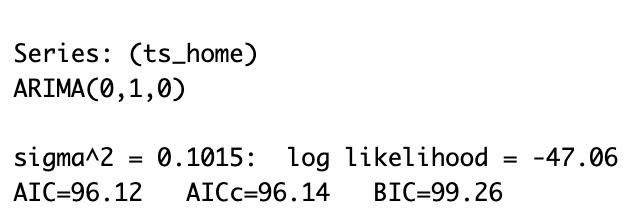
Auto Arima selected ARIMA(0,1,0)
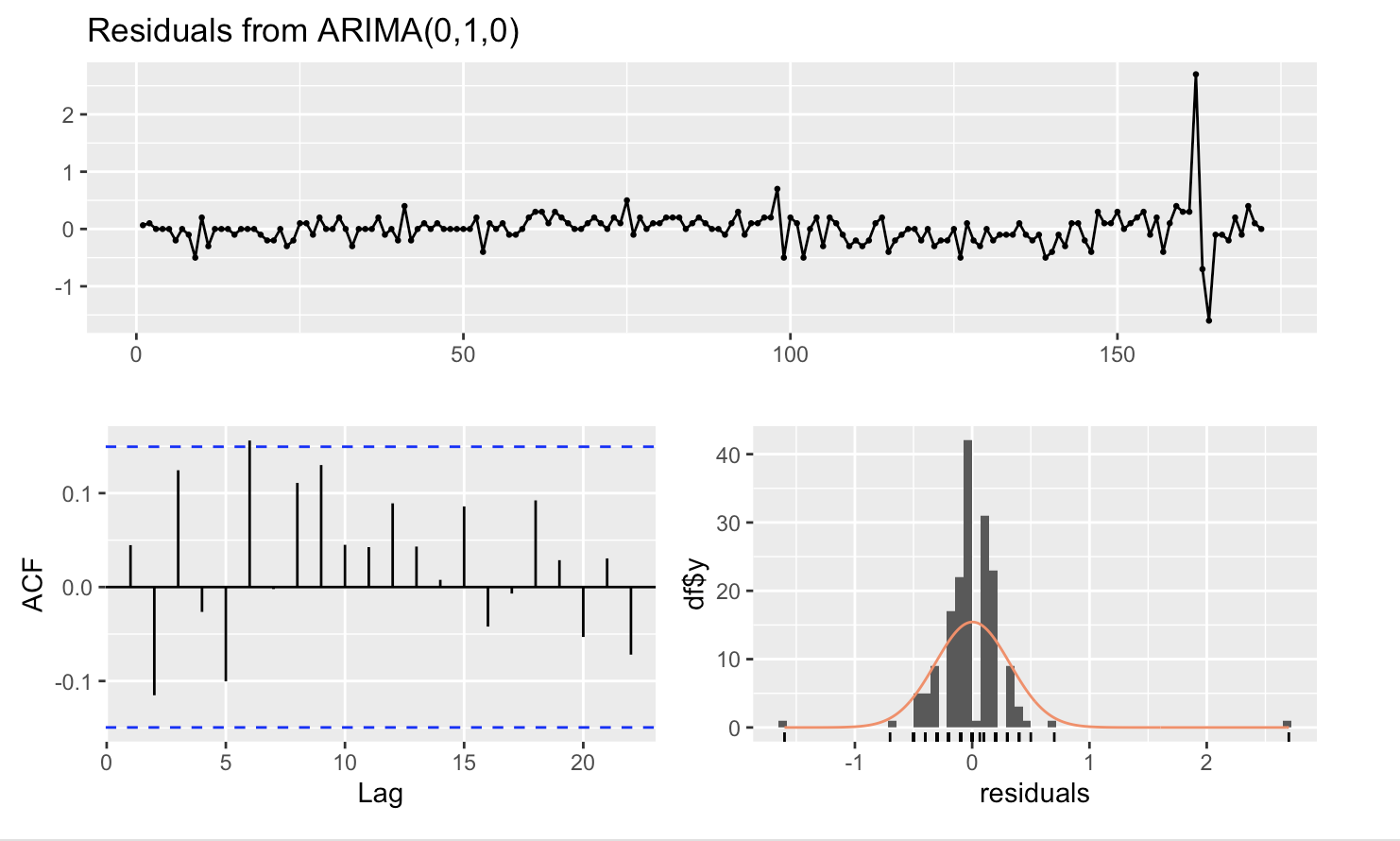
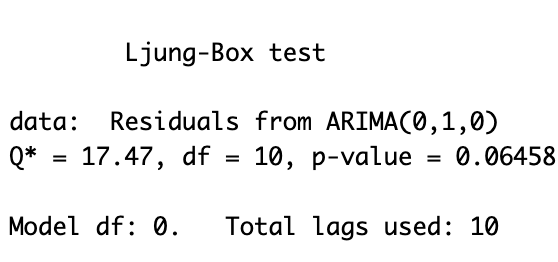
According to the residuals of the auto ARIMA model, the lags are not correlated, and the distribution of residuals follows a normal distribution. And the Ljung-Box Test tells us that it is not statistically significant at the 95%, but statistically significant at the 90%
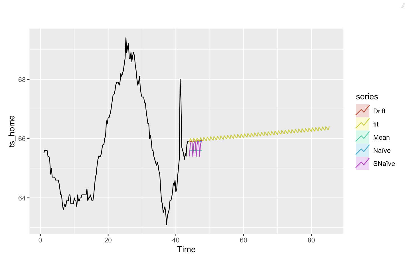
Forcast
SARIMA
SARIMA models are an extension of ARIMA models, commonly used for non-seasonal time series data. ARIMA models assume that the data is stationary, meaning that its statistical properties do not change over time. However, many time series data sets exhibit seasonal patterns, meaning that the statistical properties of the data change at regular intervals. SARIMA models are designed to capture these seasonal patterns. The "seasonal" part of SARIMA models involves additional parameters denoting the seasonal periods and their associated autoregressive, integrated, and moving average components. The seasonal component is characterized by (P, D, Q), where P denotes the seasonal autoregressive order, D represents the seasonal difference order, and Q symbolizes the seasonal moving average order.
In order to use a model such as SARMA, the time series must be stationary -one whose properties do not depend on the time at which the series is observed . the. If the time series is not stationary, we must differentiate or detrend the time series to make the series stationary. Therefore the first I model selection is first testing if the data is stationary. We do this by using the ACF plot – plots the correlation coefficient against the lag, which is measured in terms of a number of periods or units –and Augmented Dickey-Fuller (ADF) test. ADF test is used to check whether a given time series is at rest.
Figure 1a: APC Plot

Figure 1b: ACF Test

Based on the figures about, both the ACF plot and the ADF test tell us that the time series is not stationary. The ACF plot shows that the correlation among the lag variables are significant so the data is not stationary. The ADF test also agrees with the ACF test, as the p-value is greater than 0.05. Based on these results we concluded that we need to difference the time series to make it stationary.
Diffrencing Data
Figure 2a: Diffrenced Time Series

Figure 2b: ACF and PACF on Diffrenced Time Series

Figure 2c: ADF Test on Diffrenced Time Series

According to the plots above, the series is weakly stationary after the fist difference since the correlation among the lag variables are no longer significant. No more difference is needed.
Parameter Selection
Figure 3:ACF and PACF Plots for Homeownership Rates

Model Selection
In ARIMA model, AR part (p) is selected by PACF plot. After difference, lag variables are significant so p =8. MA part (q) is selected by ACF plot After difference, lag variables are significant so q = 1, 6. Since the series is derived after first difference, part I (d) = 1.
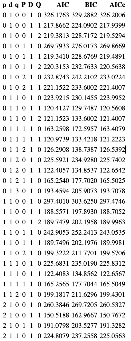
Below is a the output for the lowest AIC, BIC and AICc

As seen below the best arima model is ARIMA(0,1,1)(0,1,1).
Model Diagnostics
Figure: Model 11 Model Diagnostics
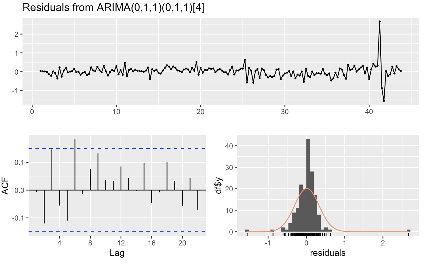
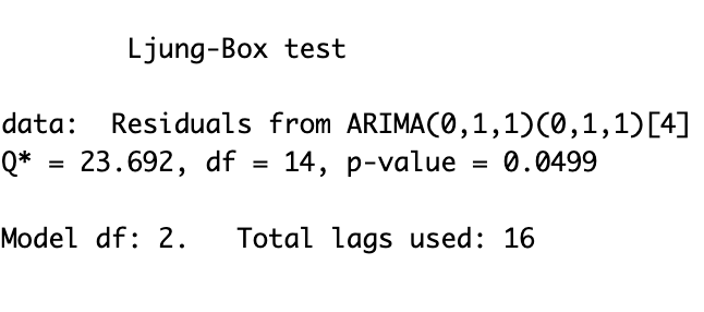
As shown below, the Ljun-Box test tells us that the p-value is .04 indicating a statistical significance.
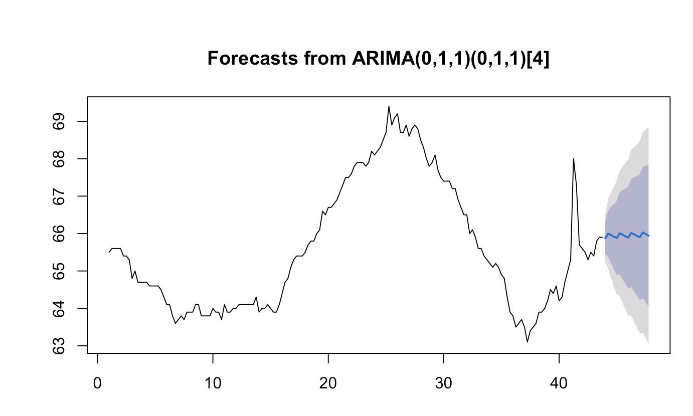
Forecast
Benchmark
